
ROKO
AE (Autoencoder) 본문
Unsupervised learning
- feed-forward neural net whose job it is to take an input x and predict x
- purpose : learning encoder

Map high dimensional data to low dimenstions representation
Learn abstract features in an unsupervised way so you can apply them to a supervised task
linear autoencoder is similar as PCA
input data에 대해 가중치 W를 곱해주는데 이걸 subspace로 projection후 basis U에 대해 표현한다고 생각하면 PCA가 되는것이다.
We will talk about nonlinear deep autoencoder
Deep nonlinear autoencoders learn to project the data onto a nonlinear subspace manifold
It is nonlinear dimension reduction

AE의 목적은 고차원의 데이터를 잘 표현하도록 하는 encoder를 얻어내는 것이다.
그러한 encoder를 학습시키기 위해 decoder를 붙여 reconstruction task를 수행하는 것인데 VAE는 생성모델이기 때문에 반대로 decoder를 얻어내는게 목적이다. 이는 VAE에서 자세하게 다루자.
𝐴 : R𝑛 → R𝑝 (encoder), 𝐵 : R𝑝 → R𝑛 (decoder) 라고 할때
argmin𝐴,𝐵 𝐸[Δ(x,𝐵◦𝐴(x)] 가 object function 이다.
input x에 대해 encoder를 거치고 다시 decoder로 reconstruct 했을때 L2 norm을 기준으로 오차가 작아지도록 학습한다.
AE의 여러가지 응용
- feature size
- undercomplete AEs (feature < input)
- overcomplete AEs (feature > input)
- Fully connected AEs
- Convolutional AEs
- etc
Regularization autoencoder
hidden이 input보다 작은경우 bottleneck으로써 low dimension representation을 잘 얻을수 있다고 믿을 수 있다. 하지만 encoder, decoder가 충분히 크다면 작은 값에서도 overfitting이 가능하다. 반대로 overcomplete AE인 경우 내부 값이 identity function과 같이 작용할 수 있기 때문에 의미있는 feature extraction을 하도록 규제를 해줘야한다.
AE에서 가장 중요한 trade off 는 bias-variance trade off이다. 우리는 학습한 latent vector가 원본 input X를 잘 reconstruct하기를 바라고 의미있는 low latent representation을 얻기를 바란다.
이런 trade off 관계를 어떻게 완화시키는지 살펴보자.
Sparse autoencoder
argmin𝐴,𝐵 𝐸[Δ(x,𝐵◦𝐴(x)]+𝜆∑︁|𝑎𝑖|
- hidden layer의 activation에 규제를 주어 sparsitfy하는 방법
argmin𝐴,𝐵 𝐸[Δ(x,𝐵◦𝐴(x)]+∑︁𝐾𝐿(𝑝||𝑝ˆ𝑗)
- 각각의 activation이 bernulli probability를 따른다고 가정하여 실제 분포와 예측 분포의 KLD값을 규제항으로 넣는 방법
Denoising autoencoder

Robust to perturbation
딥러닝은 자그마한 noise변화에도 다른 label로 분류하거나 예측하는 경우가 있다. noise에 대해 강인함을 키우기 위해 학습시에 noise를 넣어서 학습하는 방식이다.
𝐶𝜎(x ̃|x) = N(x,𝜎2I)
- input X에 white noise additive
𝐶𝑝(x ̃|x)=𝛽⊙x, 𝛽∼𝐵𝑒𝑟(𝑝)
- dropoutr과 같이 input X 일부를 drop
Contrastive autoencoder
In contractive autoencoders, the emphasis is on making the feature extraction less sensitive to small perturbations
Denoising 과 비슷하게 perturbation에 강인함을 목적으로 한것은 맞지만 targeting이 다르다. contrastive는 feature extraction에 영향을 미치는 noise에 대해 강인함을 얻기 위해 사용한다. decoder에서 reconstruction task에서 중요하지 않은 feature를 추출하지 않도록 유도하는 loss식을 정의한다.
argmin𝐴,𝐵 𝐸[Δ(𝑥,𝐵◦𝐴(𝑥)]+𝜆||𝐽𝐴(𝑥)||2
- hidden layer의 Jaccobian에 penalty를 부여하는데 이는 reconstruction error와 정반대의 효과를 유도한다.
- latent vector들간의 유사도가 증가하기에 재복원하기 어려워진다.
- 주요 포인트는 latent의 다양성은 중요하지 않고 latent가 유사해진다한들 reconstruction에 가장 많은 영향을 끼치는 latent feature extraction을 할 수 있으면 충분하다는 관점이다.
Variational autoencoder
지금까지의 autoencdoer는 encoder가 주목적이였다면 VAE는 생성모델로써 목적성을 띄고 있기에 decoder가 핵심이다. AE와 VAE는 구성이 비슷할뿐 전혀 다른 모델임을 인지하자.
Vaiational Bayes inference를 통해 확률분포를 기반으로 이미지를 생성한다.
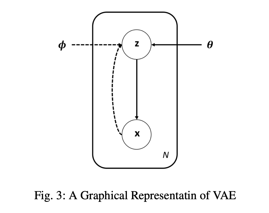
VAE의 3가지 가정
- i.i.d(identiacal and indpendent distributed) sample을 잘 표현한 조건부 latent variable을 통해 parameter\(\theta\)를 학습해 sample distribution을 표현할 수 있다. (probablistic decoder)
- parameter\(\phi\) 학습을 통해 bayes theorem을 이용해 sample이 주어졌을때 latent variable에 대한 posterior를 가정할 수 있다. (probablistic encoder)
- latent variable은 gaussian distribution을 따른다. (prior)
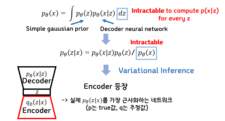
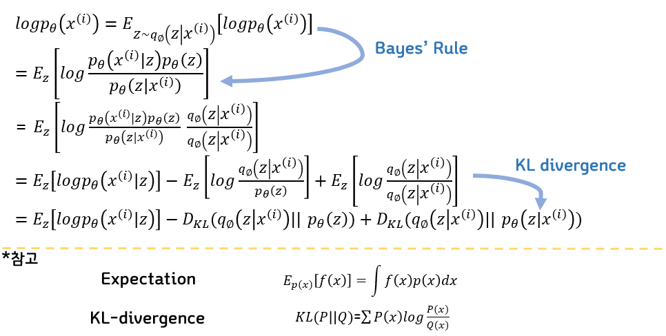
전체적인 loss식은 decoder로부터 X가 나올 최대 likelihood를 구하는데 bayes theorem을 이용해 z에 대한 식으로 변환한다. 이때 z의 분포를 알 수 없으므로 encoder를 통해 z의 분포를 학습하고 예측한다.

* ELBO에 대한 자세한 설명은 [link] 참조
ELBO 뒤의 term KLD는 최소 0 이상임을 알고 있으니 우리는 ELBO를 최대한 최대화 시키는 방향으로 학습을 진행한다.
대체로 loss function은 maximize보다 minimize방식을 채택하므로 앞부분에 -를 붙여 minimize loss function문제로 변환한다.
VAE의 특징
- Classical mean-field VB(variational Bayes) assumes a factorized approximate posterior followed by a closed form optimization updates (which usually required conjugate priors)
- VAE follows a different path using a the reparameterization trick and stochastic gradient optimization.
- With monte-carlo method, sampling z only once for each epoch.
- VAE 의 Loss 식은 ELBO를 활용한 Surrogate loss로 구성된다. (확률분포에 대한 loss를 직접적으로 구하지 않음)
Reparametrization trick
Using an auxiliary noise variable 𝜖 drawn from gaussian distribution
sampling자체는 함수로 표현될 수 없어서 back propagation이 불가하다. 하지만 임의의 𝜖 을 sampling하여 latent variable에 곱해준다면 gradient flow가 흐를수 있다. 이를 이용한 것이 재매개변수화 기법이다.
더 직관적인 해설은 [link]을 참조하자.
Disentangled autoencoder
L(𝜃,𝜙,x(𝑖))=−𝛽𝐷𝐾𝐿(𝑞𝜙(𝑧|x(𝑖))||𝑝𝜃(𝑧))+E𝑞𝜙(𝑧|x(𝑖))[log𝑝𝜃(x(𝑖)|𝑧)]
Left KLD term 에 𝛽를 곱한 형태이다. 보통 prior를 가우시안 분포로 가정하는데 가우시안 분포는 공분산이 uncorrelated한 분포이다. 따라서 𝑞와𝑝 의 분포 차이를 줄이도록 학습하므로 𝑞 또한 상관관계가 덜하도록 feature를 학습하게 되는데, 𝛽항을 가중치와 같이 큰 값으로 하게 되면 더 uncorrelated 한 independent한 feature들을 만들 수 있다.
Application of autoencoder
Generative model

Classification model
large dataset에 대해서 small dataset만 label이 전처리되어있다면 semi-supervised learning을 통해 학습을 진행시킬 수 있다. 핵심은 같은 label끼리는 비슷한 latent variable을 가저야 한다는 것이다. AE를 먼저 학습시킨뒤 encoder 부분만 classification task의 input으로 사용하면 적당히 training 과정에서 fine-tuning이 진행 될 것이다.
layer-by-layer training이 불가한 경우 nonlinearity를 적용하기 직전 각각의 layer에 대해 적용하면 closed form으로 최적해를 찾을 수 있다.
AE를 classification loss의 regularization term으로 사용하는 방식도 있다.

Clustering model
Most of the clustering algorithms are sensitive to the dimensions of the data, and suffer from the curse of dimensionality. classification처럼 학습된 AE에서 encoder만 이용해 cluster algorithm을 적용하는데, AE는 reconstruction에 대해서만 잘 작동하도록 feature learning이 되었기 때문에 clustering에는 다소 적합하지않거나 성능이 떨어질수도 있다. 이럴때는 clustering loss에 이를 tuing하기 의한 term을 넣어서 training과정중에 학습되도록 해결할 수 있다.
예를 들어 kmeans 를 사용한다면 각 cluster 중심에 거리가 가까워지도록 auxiliary term을 추가하는 것이다.
Anomaly detection
Anomaly detection is another unsupervised task.
normal dataset들에 대해서 학습 후 anomalies를 넣게 되면 reconstruction error가 크게 나오면서 anomaliy detecttion의 역할을 수행할 수 있다.
Recommendation system
In CF, user preferences are inferred based on information from other user preferences. The hidden assumption is that the human preferences are highly correlated.
사용자는 이전에 했던 소비습관을 미래에도 비슷하게 보일 확률이 높다는 가정을 이용하는 것이다.
대표적인 모델로 AutoRec이 있는데 2가지 방법론이 존재한다.
- User-based AutoRec (U-AutoRec), learn item preference for specific user
- Item-based AutoRec (I-AutoRec), learn user preference for specific item
Dimensionality reduction
The goal of dimensionality reduction is to learn a a lower dimensional manifold, so-called “intrinsic dimensionality” space.
PCA, LDA, ISOMAP 다양한 차원축소 기법이 있지만 AE가 직관적이며 비선형특징도 잘 나타낸다.
Advanced autoencoder techniques
AE는 latent variable로 활용성을 높일 수 있지만 주요한 단점은 decoder로 나온 결과물이 blurry하다. 이러한 이유는 loss function에 얼마나 사실적인지에 대한 차이값과 blur하지 않은 이미지들의 prior값이 적용되어 있지 않기 때문이다.
이런 단점들을 어떻게 해결했는지 살펴보자.
GAN (Generative adversarial network)
- gernerator vs discriminator architecture
- VAE의 KLD는 discriminator가 prior와 posterior를 비교하는 loss로 대체되었고 reconstruction error term은 generator와 연결된 discriminator에 대한 loss식으로 대체되었다.
GAN과 VAE를 결합한 모델이 사용되기도 하는데, 이는 GMM을 이용힌 latent variable inference를 가능하게 해준다.
http://dl-ai.blogspot.com/2017/08/gan-problems.html
[GAN] GAN이 풀어야 할 과제들
지금까지 GAN의 원리를 살펴봤습니다. 작동 원리를 알고나니 GAN으로 무엇이든 만들어낼 수 있을 것 같은 생각이 듭니다. 하지만 세상에 완벽한 것은 없는 법. GAN에도 아직 해결해야 할 문제점
dl-ai.blogspot.com
Adversarially learned inference (ALI)
GAN의 대표적인 문제점으로 mode collapse가 있다. generator가 고른 분포를 가진 fake data를 생성하는 것이 아닌 특정 feature에 대한 data만 반복적으로 생성하는 것이다.
ALI는 GAN과 VAE를 결합해 서로의 장단점을 보완하는것을 목표로 하는 기법이다.
VAE의 loss function 대신 encoder로부터 얻은 \((X,\hat{z})\) pair와 decoder로부터 얻은 \((\tilde{X},z)\) pair를 구분하는 discriminator의 loss를 기준으로 학습하게 된다. 이로써 decoder는 discriminator를 속이기 위해 더 현실적인 data를 생성하도록 강요받는다.
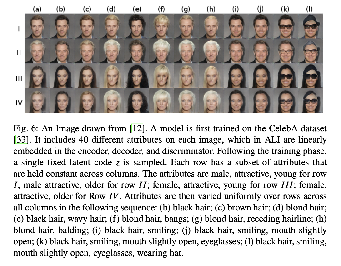
ALI는 GAN과 VAE를 결합한 방식의 초석으로 이후에 개량된 많은 모델들이 나오게 된다.
- HALI : hierachical structure로 reconstruction ability를 높이려 시도
- ALICE : add condtional entropy loss between real data and reconstruction data
Wasserstein autoencoder
ALI 에서 image를 생성하도록 강요받지만 추론하는 능력은 다소 떨어지고 내재된 학습 성능 문제가 여러가지가 있다.
W-GAN은 loss 식에 wasserstein distance(Optimal Transfer distance)를 사용하여 많은 문제를 해결했다.

WGAN에 대한 자세한 설명이 medium blogsite에 설명되어있다.
https://jonathan-hui.medium.com/gan-wasserstein-gan-wgan-gp-6a1a2aa1b490
GAN — Wasserstein GAN & WGAN-GP
Training GAN is hard. Models may never converge and mode collapses are common. To move forward, we can make incremental improvements or…
jonathan-hui.medium.com
Deep feature consistent variational autoencoder
pretrained classification model은 현재 각종 목적과 필요에 따라 효율적으로 쓰이고 있다. fine-tuning을 통해 기존 domain에서 new domain에 적용하는데, 대표적인 예시로 style-transfer가 있다. 어떠한 이미지에 다른 style의 feature를 주입시켜 이미지를 변환하는 것이다.
AE에 적용시키자면, pretrained model을 AE의 loss function을 만드는데 사용한다. original image와 reconstruction image를 input으로 넣는데, 가정이 깔려있다.
- pretrained classification model은 높은 정확도를 가지고 학습되어 있다.
- AE와 pretrained classification model의 학습된 domain의 차이가 크지 않다.
domain차이가 크지 않다는건 예를 들어 사진과 작가의 사진 차이로 보면 된다. 둘다 어떤 그림인지는 알 수 있으나 style이 다르기 때문에 domain이 살짝 다르다.
그러므로 최종 image의 차이를 loss로 학습하는 것이 아닌 pretrained classification model layer마다 feature차이를 loss로 학습한다. 그러면 AE는 더 정확하고 세밀하게 loss에 대해 학습할 수 있다.
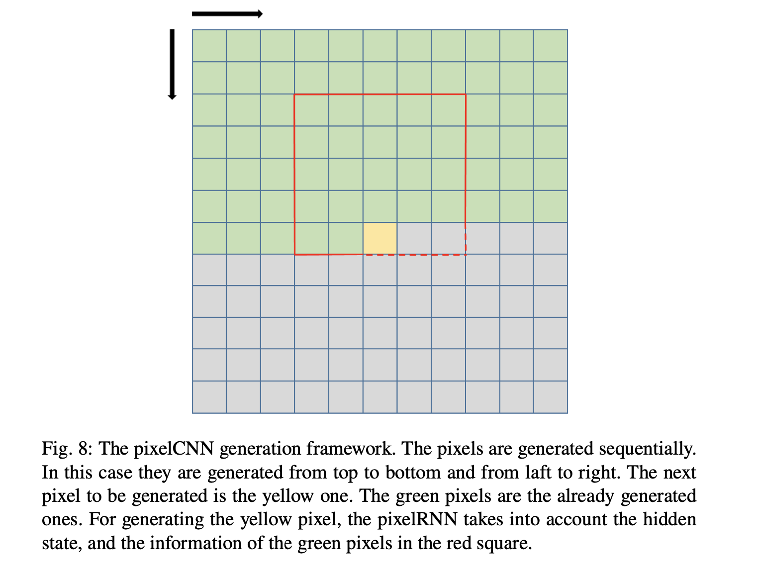
Conditional image generation with PixelCNN decoders
AE와 PixelCNN을 결합한 방식도 있다. PixelCNN은 현재까지 생성된 값과 input을 기준으로 다음 pixel값을 sequential하게 만들어 낸다. CNN을 이용해 local spatial statistic 을 이용해 전체적인 배경의 영향을 줄이고 근접해 있는 pixel을 고려하여 blurred pixel이 나타날 확률을 줄이게 된다. 이후 모델에서는 CNN이 RNN으로 대체 되었지만 핵심 contribution은 그대로 남아있다.
이제 이 RNN부분을 AE의 decoder로 대체하여 PixelCNN decoders를 만들어 낼 수 있다.
Conclusion
We would like to have a representation that is meaningful to us, and at the same time good for reconstruction. In that trade off, it is important to find the architectures which serves all needs.
https://arxiv.org/abs/2003.05991
Autoencoders
An autoencoder is a specific type of a neural network, which is mainly designed to encode the input into a compressed and meaningful representation, and then decode it back such that the reconstructed input is similar as possible to the original one. This
arxiv.org
'Artificial Intelligence > Deep Learning' 카테고리의 다른 글
| [coursera] Neural Networks and Deep Learning: Week 3 (0) | 2024.06.29 |
|---|---|
| [coursera] Neural Networks and Deep Learning: Week 2-2 (0) | 2024.06.29 |
| [coursera] Neural Networks and Deep Learning: Week 2-1 (0) | 2024.06.29 |
| [coursera] Neural Networks and Deep Learning: Week 1 (0) | 2024.06.28 |


