
ROKO
[CS234] Reinforcement Learning: Lecture 1 본문
Reinforcement learning (RL)
- Learning through experience / data to make good decisions under uncertainty
- Essential part of intelligence
- Builds strongly from theory and ideas starting in the 1950s with Richard Bellman
- A number of impressive successes in the last decade
Examples of RL

출처: https://www.nature.com/articles/nature24270%20

출처: https://openai.com/blog/chatgpt/

출처: https://arxiv.org/pdf/1709.06560.pdf
논문으로부터 나타난 히스토그램은 시간에 따른 RL 논문 증가량을 보여준다.
RL (Generally) involves
- Optimization
- Delayed consequences
- Exploration
- Generalization
Optimization은 자명하게도 최종 목적에 효율적으로 접근해야 하기에 필요한 요소이다.
Delayed consequences는 두가지 어려운 점을 가지고 있다. Planning 과정에서 당장의 이익 뿐만아니라 긴 시점에서의 이득까지 고려해야 한다는 점과 learning 과정에서 temporal reward를 어떻게 줄 것이냐는 것이다. temporal reward를 주기 어려운 이유는 당장은 이득이여도 최종 목적에 반하는 악영향을 끼치는 선택일 수 있기 때문이다.
학습 시에 선택을 할때 해당 선택에 대한 reward만 반영받게 되므로 다른 선택지들의 potential을 확인하지 못한다. Exploration은 선택 할 때마다 활용하여 확인하지 않은 선택지들도 고려하게 된다면 알지 못 할 뻔했던 최적의 선택을 발견 할 수도 있다.
RL 은 이전의 경험으로부터 학습하는데 이전 경험의 경우에 과적합 되지 않도록 generalization 하는 과정은 중요하다.
| AI Planning | Supervised Learning (SL) |
Unsupervised Learning (UL) |
Reinforcement Learning |
Imitation Learning (IL) |
|
| Optimization | v | v | v | ||
| Learns from experience | v | v | v | v | |
| Generalization | v | v | v | v | v |
| Delayed consequences | v | v | v | ||
| Exploartion | v |
IL은 RL을 SL로 바꿔주는 방식이다. IL이 좋은 많은 이유들이 있기에 유명한 방법론 중 하나이다. AI planning과 RL의 차이점이 헷갈릴 수 있다. Planning이란 단어 뜻으로 구분하면 되는데 AI planning은 모든 environment model (=transition probability)을 알고 있는 상황에서 action을 결정하는 방식이라고 생각하면된다.
Two problem categories where RL is particularly powerful
- No examples of desired behavior
- The goal is to go beyond human performance or there is no existing data for a task
- Enormous search or optimization problems with delayed outcomes
Sequential Decision Making

Goal: Select actions to maximize total expected future reward
May require balancing immediate & long term rewards
Examples

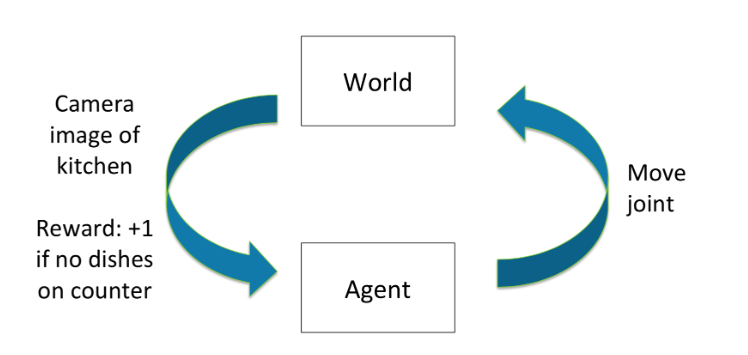
Sequential decision process (discrete time)

Each time step t:
Agent takes an action \(a_t\)
World updates given action \(a_t\), emits observation \(o_t\) and reward \(r_t\)
Agent receives observation \(o_t\) and reward \(r_t\)
History \(h_t=(a_1,o_1,r_1,\cdots,a_t,o_t,r_t)\)
Agent history로 부터 학습된 policy를 기준으로 action을 선택한다.
State is information assumed to determine what happens next
\(\rightarrow\) Function of history: \(s_t=(h_t)\)
Markov Process (MP) or Markov Chain (MC)
Markov property를 만족하는 random process를 의미한다. 이전 state만 있으면 되므로 memoryless random process이다.
Markov Reward Process (MRP)
Random process가 Markov chain 을 만족하고 rewards가 주어지는 process이다.
rewards는 1xdim(state) 벡터로 표현 할 수 있다.
Markov Assumption & Markov Decision Process
Information state: sufficient statistics of history
State \(s_t\) is Markov iff \(p(s_{t+1}|s_t,a_t)=p(s_{t+1}|h_t,a_t)\)
Future is independent if past given present
즉, 마르코프 추정은 미래에 이전 time step의 행위만 영향을 미친다는 것이다. 학습에 필요한 데이터 양을 급격하게 낮출 수 있고 계산량 감소 또한 자연스레 따라오게 되기 때문에 매우 효율적인 추정이다.
그리고 Markov property를 만족하는 decision process를 Markov Decision Process (MDP) 라고 한다.
MDP 는 state마다 Markov property를 만족하는 tuple \((S, A, P, R, \gamma)\) 이다.
- \(S\): state space
- \(A\): action space
- \(P\): transition / dynamics model
- \(R\): Reward model
- \(\gamma\): discount factor
참고로 MDP에서 decision 은 action을 결정하는걸 의미한다.
Policy
Policy \(\pi\) determines how the agent chooses actions
\(\pi:S \rightarrow A\), mapping from states to actions
Deterministic policy: \(\pi(s)=a\)
Stochastic policy: \(\pi(a|s)=Pr(a_t=a|s_t=s)\)
두 차이는 state \(s_t\)에서 최적의 action 하나를 결정하여 선택할지 가장 좋은 action을 확률적으로 선택하는 것이다.
Evaluation & Control
- Evaluation means estimate / predict the expected rewards from following a given policy
- Control is optimization (find the best policy)
Return & Value function
Horizon (H)
- number of time steps in each episode
- infinite or finite
Return, \(G_t\)
- the discounted sum of rewards from time step t to horizon H
- \(G_t=r_t+\gamma r_{t+1}+\gamma^2 r_{t+2}+\cdots+\gamma^{H-1}r_{t+H-1}\)
State Value function, \(\textbf{V(s)}\)
- Expected return from starting in state s
- \(V(s)=E[G_t|s_t=s]=E[r_t+\gamma r_{t+1}+\gamma^2 r_{t+2}+\cdots+\gamma^{H-1}r_{t+H-1}|s_t=s]=R(s)+\gamma \sum_{s' \in S}P(s'|s)V(s')\)
- \(R(s)\): immediate reward

- discount factor is usually \(\gamma < 1\), but if episode lengths are always finite (\(H < \infty\)), can use \(\gamma=1\)
- \(\gamma =0\): only care about immediate reward, \(\gamma =1\): future reward is as beneficial as immediate reward
Analytic solution of Value of an MRP
V = R + \(\gamma\)PV 방정식을 해석적으로 풀면 value function을 한번에 풀 수있기에 간단한 문제처럼 보이기도 한다.
V - \(\gamma\)PV = R
(I - \(\gamma\)P)V = R
V = \((I-\gamma P)^{-1}R\)
\((I-\gamma P)\)는 \(\gamma\), 와 \(P\)값 모두 1보다 작기 때문에 invertible하다. 하지만 역행렬을 구하는건 \(O(N^3)\)의 시간 복잡도가 소요되어 적당한 finite한 범위에서는 가능하나 값이 커지면 현실적으로 적용하기 어렵다. 따라서 값이 큰 finite 값에서도 해결하기 위해서 dynamic programming을 이용한다.
Iterative Algorithm for Computing Value of an MRP
Dynamic programming
Initialize \(V_0(s)=0\) for all s
For k=1 until convergence
For all s in S
\(V_k(s)=R(s)+\gamma\sum_{s' \in S}P(s'|s)V_{k-1}(s')\)
Computational complexity: \(O(|s|^2\) for each iteration (|s|=N)
Summary
- Reinforcement learning involves learning, optimization, delayed consequences, generalization, and exploration
- Goal is to learn to make good decisions under uncertainty
'Deep Learning' 카테고리의 다른 글
| [CS234] Reinforcement Learning: Lecture 3 (0) | 2024.07.16 |
|---|---|
| [CS234] Reinforcement Learning: Lecture 2 (0) | 2024.07.11 |
| [coursera] Sequence Models: Week 4 (0) | 2024.07.09 |
| [coursera] Sequence Models: Week 3 (0) | 2024.07.09 |


